Next: Matrices and Linear Algebra, Previous: Differential Equations [Contents][Index]
22 Numerical
- Introduction to fast Fourier transform
- Functions and Variables for fft
- Functions and Variables for FFTPACK5
- Functions for numerical solution of equations
- Introduction to numerical solution of differential equations
- Functions for numerical solution of differential equations
Next: Functions and Variables for fft, Up: Numerical [Contents][Index]
22.1 Introduction to fast Fourier transform
The fft package comprises functions for the numerical (not symbolic)
computation of the fast Fourier transform. This is limited to
sequences whit length that is a power of two. For more general
lengths, consider the fftpack5 package that supports sequences
of any length, but is most efficient if the length is a product of
small primes.
Next: Functions and Variables for FFTPACK5, Previous: Introduction to fast Fourier transform, Up: Numerical [Contents][Index]
22.2 Functions and Variables for fft
- Function: polartorect (r, t) 
-
Translates complex values of the form
r %e^(%i t)to the forma + b %i, where r is the magnitude and t is the phase. r and t are 1-dimensional arrays of the same size. The array size need not be a power of 2.The original values of the input arrays are replaced by the real and imaginary parts,
aandb, on return. The outputs are calculated asa = r cos(t) b = r sin(t)
polartorectis the inverse function ofrecttopolar.load("fft")loads this function. See alsofft.Categories: Package fft · Complex variables ·
- Function: recttopolar (a, b) 
-
Translates complex values of the form
a + b %ito the formr %e^(%i t), where a is the real part and b is the imaginary part. a and b are 1-dimensional arrays of the same size. The array size need not be a power of 2.The original values of the input arrays are replaced by the magnitude and angle,
randt, on return. The outputs are calculated asr = sqrt(a^2 + b^2) t = atan2(b, a)
The computed angle is in the range
-%pito%pi.recttopolaris the inverse function ofpolartorect.load("fft")loads this function. See alsofft.Categories: Package fft · Complex variables ·
- Function: inverse_fft (y) 
-
Computes the inverse complex fast Fourier transform. y is a list or array (named or unnamed) which contains the data to transform. The number of elements must be a power of 2. The elements must be literal numbers (integers, rationals, floats, or bigfloats) or symbolic constants, or expressions
a + b*%iwhereaandbare literal numbers or symbolic constants.inverse_fftreturns a new object of the same type as y, which is not modified. Results are always computed as floats or expressionsa + b*%iwhereaandbare floats. If bigfloat precision is needed the functionbf_inverse_fftcan be used instead as a drop-in replacement ofinverse_fftthat is slower, but supports bfloats.The inverse discrete Fourier transform is defined as follows. Let
xbe the output of the inverse transform. Then forjfrom 0 throughn - 1,x[j] = sum(y[k] exp(-2 %i %pi j k / n), k, 0, n - 1)
As there are various sign and normalization conventions possible, this definition of the transform may differ from that used by other mathematical software.
load("fft")loads this function.See also
fft(forward transform),recttopolar, andpolartorect.Examples:
Real data.
(%i1) load ("fft") $
(%i2) fpprintprec : 4 $
(%i3) L : [1, 2, 3, 4, -1, -2, -3, -4] $
(%i4) L1 : inverse_fft (L);
(%o4) [0.0, 14.49 %i - .8284, 0.0, 2.485 %i + 4.828, 0.0,
                       4.828 - 2.485 %i, 0.0, - 14.49 %i - .8284]
(%i5) L2 : fft (L1);
(%o5) [1.0, 2.0 - 2.168L-19 %i, 3.0 - 7.525L-20 %i,
4.0 - 4.256L-19 %i, - 1.0, 2.168L-19 %i - 2.0,
7.525L-20 %i - 3.0, 4.256L-19 %i - 4.0]
(%i6) lmax (abs (L2 - L));
(%o6)                       3.545L-16
Complex data.
(%i1) load ("fft") $
(%i2) fpprintprec : 4 $
(%i3) L : [1, 1 + %i, 1 - %i, -1, -1, 1 - %i, 1 + %i, 1] $
(%i4) L1 : inverse_fft (L);
(%o4) [4.0, 2.711L-19 %i + 4.0, 2.0 %i - 2.0,
- 2.828 %i - 2.828, 0.0, 5.421L-20 %i + 4.0, - 2.0 %i - 2.0,
2.828 %i + 2.828]
(%i5) L2 : fft (L1);
(%o5) [4.066E-20 %i + 1.0, 1.0 %i + 1.0, 1.0 - 1.0 %i,
1.55L-19 %i - 1.0, - 4.066E-20 %i - 1.0, 1.0 - 1.0 %i,
1.0 %i + 1.0, 1.0 - 7.368L-20 %i]
(%i6) lmax (abs (L2 - L));
(%o6)                       6.841L-17
Categories: Package fft ·
- Function: fft (x) 
-
Computes the complex fast Fourier transform. x is a list or array (named or unnamed) which contains the data to transform. The number of elements must be a power of 2. The elements must be literal numbers (integers, rationals, floats, or bigfloats) or symbolic constants, or expressions
a + b*%iwhereaandbare literal numbers or symbolic constants.fftreturns a new object of the same type as x, which is not modified. Results are always computed as floats or expressionsa + b*%iwhereaandbare floats. If bigfloat precision is needed the functionbf_fftcan be used instead as a drop-in replacement offftthat is slower, but supports bfloats. In addition if it is known that the input consists of only real values (no imaginary parts),real_fftcan be used which is potentially faster.The discrete Fourier transform is defined as follows. Let
ybe the output of the transform. Then forkfrom 0 throughn - 1,y[k] = (1/n) sum(x[j] exp(+2 %i %pi j k / n), j, 0, n - 1)
As there are various sign and normalization conventions possible, this definition of the transform may differ from that used by other mathematical software.
When the data x are real, real coefficients
aandbcan be computed such thatx[j] = sum(a[k]*cos(2*%pi*j*k/n)+b[k]*sin(2*%pi*j*k/n), k, 0, n/2)
with
a[0] = realpart (y[0])
b[0] = 0
and, for k from 1 through n/2 - 1,
a[k] = realpart (y[k] + y[n - k])
b[k] = imagpart (y[n - k] - y[k])
and
a[n/2] = realpart (y[n/2])
b[n/2] = 0
load("fft")loads this function.See also
inverse_fft(inverse transform),recttopolar, andpolartorect.. Seereal_fftfor FFTs of a real-valued input, andbf_fftandbf_real_fftfor operations on bigfloat values. Finally, for transforms of any size (but limited to float values), seefftpack5_fftandfftpack5_real_fft.Examples:
Real data.
(%i1) load ("fft") $
(%i2) fpprintprec : 4 $
(%i3) L : [1, 2, 3, 4, -1, -2, -3, -4] $
(%i4) L1 : fft (L);
(%o4) [0.0, 1.811 %i - .1036, 0.0, 0.3107 %i + .6036, 0.0,
                         0.6036 - 0.3107 %i, 0.0, (- 1.811 %i) - 0.1036]
(%i5) L2 : inverse_fft (L1);
(%o5) [1.0, 2.168L-19 %i + 2.0, 7.525L-20 %i + 3.0,
4.256L-19 %i + 4.0, - 1.0, - 2.168L-19 %i - 2.0,
- 7.525L-20 %i - 3.0, - 4.256L-19 %i - 4.0]
(%i6) lmax (abs (L2 - L));
(%o6)                       3.545L-16
Complex data.
(%i1) load ("fft") $
(%i2) fpprintprec : 4 $
(%i3) L : [1, 1 + %i, 1 - %i, -1, -1, 1 - %i, 1 + %i, 1] $
(%i4) L1 : fft (L);
(%o4) [0.5, 0.5, 0.25 %i - 0.25, (- 0.3536 %i) - 0.3536, 0.0, 0.5,
                                        (- 0.25 %i) - 0.25, 0.3536 %i + 0.3536]
(%i5) L2 : inverse_fft (L1);
(%o5) [1.0, 1.0 %i + 1.0, 1.0 - 1.0 %i, - 1.0, - 1.0, 1.0 - 1.0 %i,
                                                             1.0 %i + 1.0, 1.0]
(%i6) lmax (abs (L2 - L));
(%o6)                       0.0
Computation of sine and cosine coefficients.
(%i1) load ("fft") $
(%i2) fpprintprec : 4 $
(%i3) L : [1, 2, 3, 4, 5, 6, 7, 8] $
(%i4) n : length (L) $
(%i5) x : make_array (any, n) $
(%i6) fillarray (x, L) $
(%i7) y : fft (x) $
(%i8) a : make_array (any, n/2 + 1) $
(%i9) b : make_array (any, n/2 + 1) $
(%i10) a[0] : realpart (y[0]) $
(%i11) b[0] : 0 $
(%i12) for k : 1 thru n/2 - 1 do
   (a[k] : realpart (y[k] + y[n - k]),
    b[k] : imagpart (y[n - k] - y[k]));
(%o12)                        done
(%i13) a[n/2] : y[n/2] $
(%i14) b[n/2] : 0 $
(%i15) listarray (a);
(%o15)          [4.5, - 1.0, - 1.0, - 1.0, - 0.5]
(%i16) listarray (b);
(%o16)           [0, - 2.414, - 1.0, - .4142, 0]
(%i17) f(j) := sum (a[k]*cos(2*%pi*j*k/n) + b[k]*sin(2*%pi*j*k/n),
                    k, 0, n/2) $
(%i18) makelist (float (f (j)), j, 0, n - 1);
(%o18)      [1.0, 2.0, 3.0, 4.0, 5.0, 6.0, 7.0, 8.0]
Categories: Package fft ·
- Function: real_fft (x) 
-
Computes the fast Fourier transform of a real-valued sequence x. This is equivalent to performing
fft(x), except that only the firstN/2+1results are returned, whereNis the length of x.Nmust be power of two.No check is made that x contains only real values.
The symmetry properties of the Fourier transform of real sequences to reduce he complexity. In particular the first and last output values of
real_fftare purely real. For larger sequences,real_fftmay be computed more quickly thanfft.Since the output length is short, the normal
inverse_fftcannot be directly used. Useinverse_real_fftto compute the inverse.Categories: Package fft ·
- Function: inverse_real_fft (y) 
Computes the inverse Fourier transform of y, which must have a length of
N/2+1whereNis a power of two. That is, the input x is expected to be the output ofreal_fft.No check is made to ensure that the input has the correct format. (The first and last elements must be purely real.)
Categories: Package fft ·
- Function: bf_inverse_fft (y) 
-
Computes the inverse complex fast Fourier transform. This is the bigfloat version of
inverse_fftthat converts the input to bigfloats and returns a bigfloat result.Categories: Package fft ·
- Function: bf_fft (y) 
-
Computes the forward complex fast Fourier transform. This is the bigfloat version of
fftthat converts the input to bigfloats and returns a bigfloat result.Categories: Package fft ·
- Function: bf_real_fft (x) 
-
Computes the forward fast Fourier transform of a real-valued input returning a bigfloat result. This is the bigfloat version of
real_fft.Categories: Package fft ·
- Function: bf_inverse_real_fft (y) 
Computes the inverse fast Fourier transform with a real-valued bigfloat output. This is the bigfloat version of
inverse_real_fft.Categories: Package fft ·
Next: Functions for numerical solution of equations, Previous: Functions and Variables for fft, Up: Numerical [Contents][Index]
22.3 Functions and Variables for FFTPACK5
FFTPACK5 provides several routines to compute Fourier
transforms for both real and complex sequences and their inverses.
The forward transform is defined the same as for fft. The
major difference is the length of the sequence is not constrained to
be a power of two. In fact, any length is supported, but it is most
efficient when the length has the form 2^r*3^s*5^t.
load("fftpack5") loads this function.
- Function: fftpack5_fft (x) 
-
Like
fft(fft), this computes the fast Fourier transform of a complex sequence. However, the length of x is not limited to a power of 2.load("fftpack5")loads this function.Examples:
Real data.
(%i1) load("fftpack5") $
(%i2) fpprintprec : 4 $
(%i3) L : [1, 2, 3, 4, -1, -2 ,-3, -4] $
(%i4) L1 : fftpack5_fft(L);
(%o4) [0.0, 1.811 %i - 0.1036, 0.0, 0.3107 %i + 0.6036, 0.0,
                                0.6036 - 0.3107 %i, 0.0, (- 1.811 %i) - 0.1036]
(%i5) L2 : fftpack5_inverse_fft(L1);
(%o5) [1.0, 4.441e-16 %i + 2.0, 1.837e-16 %i + 3.0, 4.0 - 4.441e-16 %i,
     - 1.0, (- 4.441e-16 %i) - 2.0, (- 1.837e-16 %i) - 3.0, 4.441e-16
       %i - 4.0]
(%i6) lmax (abs (L2-L));
(%o6)                       4.441e-16
(%i7) L : [1, 2, 3, 4, 5, 6]$
(%i8) L1 : fftpack5_fft(L);
(%o8) [3.5, (- 0.866 %i) - 0.5, (- 0.2887 %i) - 0.5, (- 1.48e-16 %i) - 0.5,
                                               0.2887 %i - 0.5, 0.866
                                                      %%i - 0.5]
(%i9) L2 : fftpack5_inverse_fft (L1);
(%o9) [1.0 - 1.48e-16 %i, 3.701e-17 %i + 2.0, 3.0 - 1.48e-16 %i,
                     4.0 - 1.811e-16 %i, 5.0 - 1.48e-16 %i, 5.881e-16
                           %i + 6.0]
(%i10) lmax (abs (L2-L));
(%o10)                             9.064e-16
Complex data.
(%i1) load("fftpack5") $
(%i2) fpprintprec : 4 $
(%i3) L : [1, 1 + %i, 1 - %i, -1, -1, 1 - %i, 1 + %i, 1] $
(%i4) L1 : fftpack5_inverse_fft (L);
(%o4) [4.0, 2.828 %i + 2.828, (- 2.0 %i) - 2.0, 4.0, 0.0,
                                       (- 2.828 %i) - 2.828, 2.0 %i - 2.0, 4.0]
(%i5) L2 : fftpack5_fft(L1);
(%o5) [1.0, 1.0 %i + 1.0, 1.0 - 1.0 %i, (- 2.776e-17 %i) - 1.0, - 1.0,
                                1.0 - 1.0 %i, 1.0 %i + 1.0, 1.0 -
                                          %2.776e-17 %i]
(%i6) lmax(abs(L2-L));
(%o6)                              1.11e-16
Categories: Package fftpack5 ·
- Function: fftpack5_inverse_fft (y) 
-
Computes the inverse complex Fourier transform, like
inverse_fft, but is not constrained to be a power of two.Categories: Package fftpack5 ·
- Function: fftpack5_real_fft (x) 
-
Computes the fast Fourier transform of a real-valued sequence x, just like
real_fft, except the length is not constrained to be a power of two.Examples:
(%i1) fpprintprec : 4 $
(%i2) L : [1, 2, 3, 4, 5, 6] $
(%i3) L1 : fftpack5_real_fft(L);
(%o3)       [3.5, (- 0.866 %i) - 0.5, (- 0.2887 %i) - 0.5, - 0.5]
(%i4) L2 : fftpack5_inverse_real_fft(L1, 6);
(%o4)                  [1.0, 2.0, 3.0, 4.0, 5.0, 6.0]
(%i5) lmax(abs(L2-L));
(%o5)                            1.332e-15
(%i6) fftpack5_inverse_real_fft(L1, 7);
(%o6)            [0.5, 2.083, 2.562, 3.7, 4.3, 5.438, 5.917]
The last example shows how important it to set the length correctly for
fftpack5_inverse_real_fft.Categories: Package fftpack5 ·
- Function: fftpack5_inverse_real_fft (y, n) 
-
Computes the inverse Fourier transform of y, which must have a length of
floor(n/2) + 1. The length of sequence produced by the inverse transform must be specified by n. This is required because the length of y does not uniquely determine n. The last element of y is always real if n is even, but it can be complex when n is odd.Categories: Package fftpack5 ·
Next: Introduction to numerical solution of differential equations, Previous: Functions and Variables for FFTPACK5, Up: Numerical [Contents][Index]
22.4 Functions for numerical solution of equations
- Function: horner
horner (expr, x)
horner (expr) ¶ -
Returns a rearranged representation of expr as in Horner’s rule, using x as the main variable if it is specified.
xmay be omitted in which case the main variable of the canonical rational expression form of expr is used.hornersometimes improves stability ifexpris to be numerically evaluated. It is also useful if Maxima is used to generate programs to be run in Fortran. See alsostringout.(%i1) expr: 1e-155*x^2 - 5.5*x + 5.2e155; 2 (%o1) 1.e-155 x - 5.5 x + 5.2e+155 (%i2) expr2: horner (%, x), keepfloat: true; (%o2) 1.0 ((1.e-155 x - 5.5) x + 5.2e+155) (%i3) ev (expr, x=1e155); Maxima encountered a Lisp error: arithmetic error FLOATING-POINT-OVERFLOW signalled Automatically continuing. To enable the Lisp debugger set *debugger-hook* to nil. (%i4) ev (expr2, x=1e155); (%o4) 7.00000000000001e+154Categories: Numerical methods ·
- Function: find_root (expr, x, a, b, [abserr, relerr]) 
- Function: find_root (f, a, b, [abserr, relerr]) 
- Function: bf_find_root (expr, x, a, b, [abserr, relerr]) 
- Function: bf_find_root (f, a, b, [abserr, relerr]) 
- Option variable: find_root_error 
- Option variable: find_root_abs 
- Option variable: find_root_rel 
-
Finds a root of the expression expr or the function f over the closed interval [a, b]. The expression expr may be an equation, in which case
find_rootseeks a root oflhs(expr) - rhs(expr).Given that Maxima can evaluate expr or f over [a, b] and that expr or f is continuous,
find_rootis guaranteed to find the root, or one of the roots if there is more than one.find_rootinitially applies binary search. If the function in question appears to be smooth enough,find_rootapplies linear interpolation instead.bf_find_rootis a bigfloat version offind_root. The function is computed using bigfloat arithmetic and a bigfloat result is returned. Otherwise,bf_find_rootis identical tofind_root, and the following description is equally applicable tobf_find_root.The accuracy of
find_rootis governed byabserrandrelerr, which are optional keyword arguments tofind_root. These keyword arguments take the formkey=val. The keyword arguments areabserrDesired absolute error of function value at root. Default is
find_root_abs.relerrDesired relative error of root. Default is
find_root_rel.
find_rootstops when the function in question evaluates to something less than or equal toabserr, or if successive approximants x_0, x_1 differ by no more thanrelerr * max(abs(x_0), abs(x_1)). The default values offind_root_absandfind_root_relare both zero.find_rootexpects the function in question to have a different sign at the endpoints of the search interval. When the function evaluates to a number at both endpoints and these numbers have the same sign, the behavior offind_rootis governed byfind_root_error. Whenfind_root_erroristrue,find_rootprints an error message. Otherwisefind_rootreturns the value offind_root_error. The default value offind_root_erroristrue.If f evaluates to something other than a number at any step in the search algorithm,
find_rootreturns a partially-evaluatedfind_rootexpression.The order of a and b is ignored; the region in which a root is sought is [min(a, b), max(a, b)].
Examples:
(%i1) f(x) := sin(x) - x/2;
                                        x
(%o1)                  f(x) := sin(x) - -
                                        2
(%i2) find_root (sin(x) - x/2, x, 0.1, %pi);
(%o2)                   1.895494267033981
(%i3) find_root (sin(x) = x/2, x, 0.1, %pi);
(%o3)                   1.895494267033981
(%i4) find_root (f(x), x, 0.1, %pi);
(%o4)                   1.895494267033981
(%i5) find_root (f, 0.1, %pi);
(%o5)                   1.895494267033981
(%i6) find_root (exp(x) = y, x, 0, 100);
                            x
(%o6)           find_root(%e  = y, x, 0.0, 100.0)
(%i7) find_root (exp(x) = y, x, 0, 100), y = 10;
(%o7)                   2.302585092994046
(%i8) log (10.0);
(%o8)                   2.302585092994046
(%i9) fpprec:32;
(%o9)                           32
(%i10) bf_find_root (exp(x) = y, x, 0, 100), y = 10;
(%o10)                  2.3025850929940456840179914546844b0
(%i11) log(10b0);
(%o11)                  2.3025850929940456840179914546844b0
Categories: Algebraic equations · Numerical methods ·
- Function: newton (expr, x, x_0, eps) 
-
Returns an approximate solution of
expr = 0by Newton’s method, considering expr to be a function of one variable, x. The search begins withx = x_0and proceeds untilabs(expr) < eps(with expr evaluated at the current value of x).newtonallows undefined variables to appear in expr, so long as the termination testabs(expr) < epsevaluates totrueorfalse. Thus it is not necessary that expr evaluate to a number.load("newton1")loads this function.See also
realroots,allroots,find_rootandmnewton.Examples:
(%i1) load ("newton1");
(%o1)  /maxima/share/numeric/newton1.mac
(%i2) newton (cos (u), u, 1, 1/100);
(%o2)                   1.570675277161251
(%i3) ev (cos (u), u = %);
(%o3)                 1.2104963335033529e-4
(%i4) assume (a > 0);
(%o4)                        [a > 0]
(%i5) newton (x^2 - a^2, x, a/2, a^2/100);
(%o5)                  1.00030487804878 a
(%i6) ev (x^2 - a^2, x = %);
                                           2
(%o6)                6.098490481853958e-4 a
Categories: Algebraic equations · Numerical methods ·
Next: Functions for numerical solution of differential equations, Previous: Functions for numerical solution of equations, Up: Numerical [Contents][Index]
22.5 Introduction to numerical solution of differential equations
The Ordinary Differential Equations (ODE) solved by the functions in this section should have the form,
       dy
       -- = F(x,y)
       dx
which is a first-order ODE. Higher order differential equations of order n must be written as a system of n first-order equations of that kind. For instance, a second-order ODE should be written as a system of two equations
       dx               dy
       -- = G(x,y,t)    -- = F(x,y,t)
       dt               dt
The first argument in the functions will be a list with the expressions on the right-side of the ODE’s. The variables whose derivatives are represented by those expressions should be given in a second list. In the case above those variables are x and y. The independent variable, t in the examples above, might be given in a separated option. If the expressions given do not depend on that independent variable, the system is called autonomous.
Previous: Introduction to numerical solution of differential equations, Up: Numerical [Contents][Index]
22.6 Functions for numerical solution of differential equations
- Function: plotdf
plotdf (dydx, options…)
plotdf (dvdu, [u,v], options…)
plotdf ([dxdt,cdydt], options…)
plotdf ([dudt,cdvdt], [u,cv], options…) ¶ -
The function
plotdfcreates a two-dimensional plot of the direction field (also called slope field) for a first-order Ordinary Differential Equation (ODE) or a system of two autonomous first-order ODE’s.Plotdf requires Xmaxima, even if its run from a Maxima session in a console, since the plot will be created by the Tk scripts in Xmaxima. If Xmaxima is not installed plotdf will not work.
dydx, dxdt and dydt are expressions that depend on x and y. dvdu, dudt and dvdt are expressions that depend on u and v. In addition to those two variables, the expressions can also depend on a set of parameters, with numerical values given with the
parametersoption (the option syntax is given below), or with a range of allowed values specified by a sliders option.Several other options can be given within the command, or selected in the menu. Integral curves can be obtained by clicking on the plot, or with the option
trajectory_at. The direction of the integration can be controlled with thedirectionoption, which can have values of forward, backward or both. The number of integration steps is given bynsteps; at each integration step the time increment will be adjusted automatically to produce displacements much smaller than the size of the plot window. The numerical method used is 4th order Runge-Kutta with variable time steps.Plot window menu:
The menu bar of the plot window has the following seven icons:
An X. Can be used to close the plot window.
A wrench and a screwdriver. Opens the configuration menu with several fields that show the ODE(s) in use and various other settings. If a pair of coordinates are entered in the field Trajectory at and the enter key is pressed, a new integral curve will be shown, in addition to the ones already shown.
Two arrows following a circle. Replots the direction field with the new settings defined in the configuration menu and replots only the last integral curve that was previously plotted.
Hard disk drive with an arrow. Used to save a copy of the plot, in Postscript format, in the file specified in a field of the box that appears when that icon is clicked.
Magnifying glass with a plus sign. Zooms in the plot.
Magnifying glass with a minus sign. Zooms out the plot. The plot can be displaced by holding down the right mouse button while the mouse is moved.
Icon of a plot. Opens another window with a plot of the two variables in terms of time, for the last integral curve that was plotted.
Plot options:
Options can also be given within the
plotdfitself, each one being a list of two or more elements. The first element in each option is the name of the option, and the remainder is the value or values assigned to the option.The options which are recognized by
plotdfare the following:- nsteps defines the number of steps that will be used for the independent variable, to compute an integral curve. The default value is 100.
- direction defines the direction of the independent
variable that will be followed to compute an integral curve. Possible
values are
forward, to make the independent variable increasenstepstimes, with incrementststep,backward, to make the independent variable decrease, orboththat will lead to an integral curve that extendsnstepsforward, andnstepsbackward. The keywordsrightandleftcan be used as synonyms forforwardandbackward. The default value isboth. - tinitial defines the initial value of variable t used to compute integral curves. Since the differential equations are autonomous, that setting will only appear in the plot of the curves as functions of t. The default value is 0.
- versus_t is used to create a second plot window, with a
plot of an integral curve, as two functions x, y, of the
independent variable t. If
versus_tis given any value different from 0, the second plot window will be displayed. The second plot window includes another menu, similar to the menu of the main plot window. The default value is 0. - trajectory_at defines the coordinates xinitial and yinitial for the starting point of an integral curve. The option is empty by default.
- parameters defines a list of parameters, and their
numerical values, used in the definition of the differential
equations. The name and values of the parameters must be given in a
string with a comma-separated sequence of pairs
name=value. - sliders defines a list of parameters that will be changed
interactively using slider buttons, and the range of variation of those
parameters. The names and ranges of the parameters must be given in a
string with a comma-separated sequence of elements
name=min:max - xfun defines a string with semi-colon-separated sequence of functions of x to be displayed, on top of the direction field. Those functions will be parsed by Tcl and not by Maxima.
- x should be followed by two numbers, which will set up the minimum and maximum values shown on the horizontal axis. If the variable on the horizontal axis is not x, then this option should have the name of the variable on the horizontal axis. The default horizontal range is from -10 to 10.
- y should be followed by two numbers, which will set up the minimum and maximum values shown on the vertical axis. If the variable on the vertical axis is not y, then this option should have the name of the variable on the vertical axis. The default vertical range is from -10 to 10.
- xaxislabel will be used to identify the horizontal axis. Its default value is the name of the first state variable.
- yaxislabel will be used to identify the vertical axis. Its default value is the name of the second state variable.
- number_of_arrows should be set to a square number and defines the approximate density of the arrows being drawn. The default value is 225.
Examples:
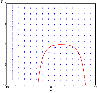
- To show the direction field of the differential equation y' = exp(-x) + y and the solution that goes through (2, -0.1):
(%i1) plotdf(exp(-x)+y,[trajectory_at,2,-0.1])$
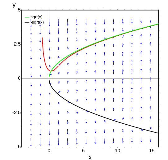
- To obtain the direction field for the equation diff(y,x) = x - y^2 and the solution with initial condition y(-1) = 3, we can use the command:
(%i1) plotdf(x-y^2,[xfun,"sqrt(x);-sqrt(x)"],
         [trajectory_at,-1,3], [direction,forward],
         [y,-5,5], [x,-4,16])$
The graph also shows the function y = sqrt(x).
- The following example shows the direction field of a harmonic oscillator,
defined by the two equations dz/dt = v and dv/dt = -k*z/m,
and the integral curve through (z,v) = (6,0), with a slider that
will allow you to change the value of m interactively (k is
fixed at 2):
(%i1) plotdf([v,-k*z/m], [z,v], [parameters,"m=2,k=2"],
           [sliders,"m=1:5"], [trajectory_at,6,0])$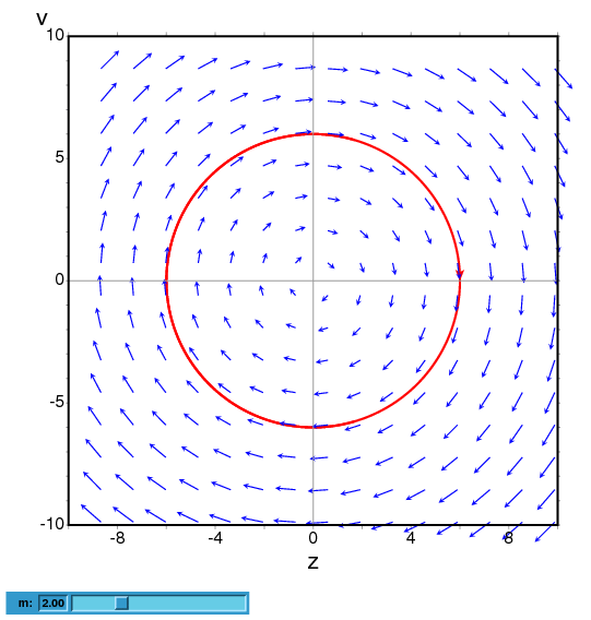
- To plot the direction field of the Duffing equation, m*x''+c*x'+k*x+b*x^3 = 0, we introduce the variable y=x' and use:
(%i1) plotdf([y,-(k*x + c*y + b*x^3)/m],
             [parameters,"k=-1,m=1.0,c=0,b=1"],
             [sliders,"k=-2:2,m=-1:1"],[tstep,0.1])$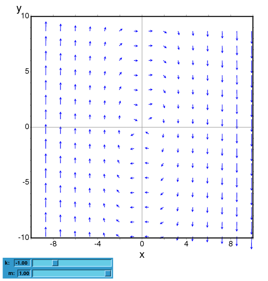
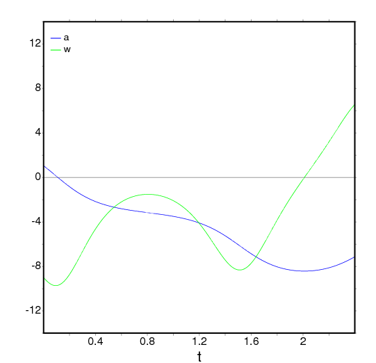
- The direction field for a damped pendulum, including the
solution for the given initial conditions, with a slider that
can be used to change the value of the mass m, and with a plot of
the two state variables as a function of time:
(%i1) plotdf([w,-g*sin(a)/l - b*w/m/l], [a,w],
        [parameters,"g=9.8,l=0.5,m=0.3,b=0.05"],
        [trajectory_at,1.05,-9],[tstep,0.01],
        [a,-10,2], [w,-14,14], [direction,forward],
        [nsteps,300], [sliders,"m=0.1:1"], [versus_t,1])$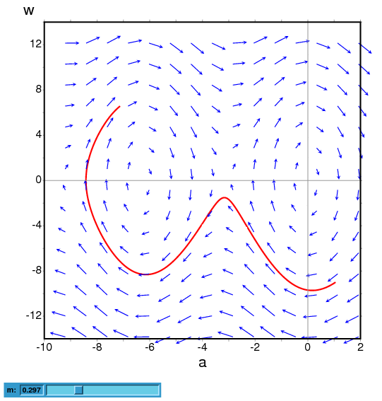
- Function: ploteq (exp, ...options...) 
-
Plots equipotential curves for exp, which should be an expression depending on two variables. The curves are obtained by integrating the differential equation that define the orthogonal trajectories to the solutions of the autonomous system obtained from the gradient of the expression given. The plot can also show the integral curves for that gradient system (option fieldlines).
This program also requires Xmaxima, even if its run from a Maxima session in a console, since the plot will be created by the Tk scripts in Xmaxima. By default, the plot region will be empty until the user clicks in a point (or gives its coordinate with in the set-up menu or via the trajectory_at option).
Most options accepted by plotdf can also be used for ploteq and the plot interface is the same that was described in plotdf.
Example:
(%i1) V: 900/((x+1)^2+y^2)^(1/2)-900/((x-1)^2+y^2)^(1/2)$
(%i2) ploteq(V,[x,-2,2],[y,-2,2],[fieldlines,"blue"])$
Clicking on a point will plot the equipotential curve that passes by that point (in red) and the orthogonal trajectory (in blue).
- Function: rk
rk (ODE, var, initial, domain)
rk ([ODE1, …, ODEm], [v1, …, vm], [init1, …, initm], domain) ¶ -
The first form solves numerically one first-order ordinary differential equation, and the second form solves a system of m of those equations, using the 4th order Runge-Kutta method. var represents the dependent variable. ODE must be an expression that depends only on the independent and dependent variables and defines the derivative of the dependent variable with respect to the independent variable.
The independent variable is specified with
domain, which must be a list of four elements as, for instance:[t, 0, 10, 0.1]
the first element of the list identifies the independent variable, the second and third elements are the initial and final values for that variable, and the last element sets the increments that should be used within that interval.
If m equations are going to be solved, there should be m dependent variables v1, v2, ..., vm. The initial values for those variables will be init1, init2, ..., initm. There will still be just one independent variable defined by
domain, as in the previous case. ODE1, ..., ODEm are the expressions that define the derivatives of each dependent variable in terms of the independent variable. The only variables that may appear in those expressions are the independent variable and any of the dependent variables. It is important to give the derivatives ODE1, ..., ODEm in the list in exactly the same order used for the dependent variables; for instance, the third element in the list will be interpreted as the derivative of the third dependent variable.The program will try to integrate the equations from the initial value of the independent variable until its last value, using constant increments. If at some step one of the dependent variables takes an absolute value too large, the integration will be interrupted at that point. The result will be a list with as many elements as the number of iterations made. Each element in the results list is itself another list with m+1 elements: the value of the independent variable, followed by the values of the dependent variables corresponding to that point.
See also
drawdf,desolveandode2.Examples:
To solve numerically the differential equation
dx/dt = t - x^2
With initial value x(t=0) = 1, in the interval of t from 0 to 8 and with increments of 0.1 for t, use:
(%i1) results: rk(t-x^2,x,1,[t,0,8,0.1])$
(%i2) plot2d ([discrete, results])$
the results will be saved in the list
resultsand the plot will show the solution obtained, with t on the horizontal axis and x on the vertical axis.To solve numerically the system:
dx/dt = 4-x^2-4*y^2 dy/dt = y^2-x^2+1
for t between 0 and 4, and with values of -1.25 and 0.75 for x and y at t=0:
(%i1) sol: rk([4-x^2-4*y^2, y^2-x^2+1], [x, y], [-1.25, 0.75],
              [t, 0, 4, 0.02])$
(%i2) plot2d([discrete, makelist([p[1], p[3]], p, sol)], [xlabel, "t"],
             [ylabel, "y"])$
The plot will show the solution for variable y as a function of t.
Categories: Differential equations · Numerical methods ·