[ < ] [ > ]   [ << ] [ Up ] [ >> ]         [Top] [Contents] [Index] [ ? ]

12. Plotting


[ < ] [ > ]   [ << ] [ Up ] [ >> ]         [Top] [Contents] [Index] [ ? ]

12.1 Introduction to Plotting

Maxima uses an external plotting package to make the plots (see the section on Plotting Formats). The plotting functions calculate a set of points and pass them to the plotting package together with a set of commands. That information can be passed to the external program either through a pipe or by calling the program with the name of a file where the data has been saved. The data file is given the name maxout_xxx.format, where xxx is a number that is unique to every concurrently-running instance of maxima and format is the name of the plotting format being used (gnuplot, xmaxima, mgnuplot or gnuplot_pipes).

There are to save the plot in a graphic format file. In those cases, the file maxout_xxx.format created by Maxima includes commands that will make the external plotting program save the result in a graphic file. The default name for that graphic file is maxplot.extension, where extension is the extension normally used for the kind of graphic file selected.

The maxout_xxx.format and maxplot.extension files are created in the directory specified by the system variable maxima_tempdir. That location can be changed by assigning to that variable (or to the environment variable MAXIMA_TEMPDIR) a string that represents a valid directory where Maxima can create new files. The output of the Maxima plotting command will be a list with the names of the file(s) created, including their complete path.

If the format used is either gnuplot or xmaxima, the external programs gnuplot or xmaxima can be run, giving it the file maxout_xxx.format as argument, in order to view again a plot previously created in Maxima. Thus, when a Maxima plotting command fails, the format can be set to gnuplot or xmaxima and the plain-text file maxout_xxx.gnuplot (or maxout_xxx.xmaxima) can be inspected to look for the source of the problem.

The additional package draw provides functions similar to the ones described in this section with some extra features. Note that some plotting options have the same name in both plotting packages, but their syntax and behavior is different. To view the documentation for a graphic option opt, type ?? opt in order to choose the information for either of those two packages.

Categories:  Plotting


[ < ] [ > ]   [ << ] [ Up ] [ >> ]         [Top] [Contents] [Index] [ ? ]

12.2 Plotting Formats

Maxima can use either Gnuplot or Xmaxima as graphics program. Gnuplot is an external program that has to be installed separately, while Xmaxima is distributed with Maxima. There are various different formats for those programs, which can be selected with the option plot_format (see also the Plotting Options section).

The plotting formats are the following:

Categories:  Plotting


[ < ] [ > ]   [ << ] [ Up ] [ >> ]         [Top] [Contents] [Index] [ ? ]

12.3 Functions and Variables for Plotting

Function: contour_plot (expr, x_range, y_range, options, …)

It plots the contours (curves of equal value) of expr over the region x_range by y_range. Any additional arguments are treated the same as in plot3d.

This function only works when the plot format is either gnuplot or gnuplot_pipes. The additional package implicit_plot, which works in any graphic format, can also be used to plot contours but a separate expression must be given for each contour.

Examples:

(%i1) contour_plot (x^2 + y^2, [x, -4, 4], [y, -4, 4])$

figures/plotting1

You can add any options accepted by plot3d; for instance, the option legend with a value of false, to remove the legend. By default, Gnuplot chooses and displays 3 contours. To increase the number of contours, it is necessary to use a custom gnuplot_preamble, as in the next example:

(%i1) contour_plot (u^3 + v^2, [u, -4, 4], [v, -4, 4],
              [legend,false],
              [gnuplot_preamble, "set cntrparam levels 12"])$

figures/plotting2

Categories:  Plotting

Function: get_plot_option (keyword, index)

Returns the current default value of the option named keyword, which is a list. The optional argument index must be a positive integer which can be used to extract only one element from the list (element 1 is the name of the option).

See also set_plot_option, remove_plot_option and the section on Plotting Options.

System variable: gnuplot_command

This variable stores the name of the command used to run the gnuplot program when the plot format is gnuplot. Its default value is "wgnuplot" in Windows and "gnuplot" in other systems. If the gnuplot program is not found unless you give its complete path or if you want to try a different version of it, you may change the value of this variable. For instance,

(%i1) gnuplot_command: "/usr/local/bin/my_gnuplot"$

Categories:  Plotting

System variable: gnuplot_file_args

When a graphic file is going to be created using gnuplot, this variable is used to specify the way the file name should be passed to gnuplot. Its default value is "~s", which means that the name of the file will be passed directly. The contents of this variable can be changed in order to add options for the gnuplot program, adding those options before the format directive "~s".

Categories:  Plotting

System variable: gnuplot_view_args

This variable is used to parse the argument that will be passed to the gnuplot program when the plot format is gnuplot. Its default value is "-persist ~s", where "~s" will be replaced with the name of the file where the gnuplot commands have been written (usually "maxout_xxx.gnuplot"). The option -persist tells gnuplot to exit after the commands in the file have been executed, without closing the window that displays the plot.

Those familiar with gnuplot, might want to change the value of this variable. For example, by changing it to:

(%i1) gnuplot_view_args: "~s -"$

gnuplot will not be closed after the commands in the file have been executed; thus, the window with the plot will remain, as well as the gnuplot interactive shell where other commands can be issued in order to modify the plot.

In Windows versions of Gnuplot older than 4.6.3 the behavior of "~s -" and "-persist ~s" were the opposite; namely, "-persist ~s" made the plot window and the gnuplot interactive shell remain, while "~s -" closed the gnuplot shell keeping the plot window. Therefore, when older gnuplot versions are used in Windows, it might be necessary to adjust the value of gnuplot_view_args.

Categories:  Plotting

Function: implicit_plot  
    implicit_plot (expr, x_range, y_range)  
    implicit_plot ([expr_1, …, expr_n], x_range, y_range)

Displays a plot of a function on the real plane, defined implicitly by the expression expr. The domain in the plane is defined by x_range and y_range. Several functions can be represented on the same plot, giving a list [expr_1, …, expr_n] of expressions that define them. This function uses the global format options set up with the set_plot_option. Additional options can also be given as extra arguments for the implicit_plot command.

The method used by implicit_plot consists of tracking sign changes on the domain given and it can fail for complicated expressions.

load(implicit_plot) loads this function.

Example:

(%i1) load(implicit_plot)$
(%i2) implicit_plot (x^2 = y^3 - 3*y + 1, [x, -4, 4], [y, -4, 4])$

figures/plotting3

Function: julia (x, y, ...options...)

Creates a graphic representation of the Julia set for the complex number (x + i y). The two mandatory parameters x and y must be real. This program is part of the additional package dynamics, but that package does not have to be loaded; the first time julia is used, it will be loaded automatically.

Each pixel in the grid is given a color corresponding to the number of iterations it takes the sequence that starts at that point to move out of the convergence circle of radius 2 centered at the origin. The number of pixels in the grid is controlled by the grid plot option (default 30 by 30). The maximum number of iterations is set with the option iterations. The program uses its own default palette: magenta,violet, blue, cyan, green, yellow, orange, red, brown and black, but it can be changed by adding an explicit palette option in the command.

The default domain used goes from -2 to 2 in both axes and can be changed with the x and y options. By default, the two axes are shown with the same scale, unless the option yx_ratio is used or the option same_xy is disabled. Other general plot options are also accepted.

The following example shows a region of the Julia set for the number -0.55 + i0.6. The option color_bar_tics is used to prevent Gnuplot from adjusting the color box up to 40, in which case the points corresponding the maximum 36 iterations would not be black.

(%i1) julia (-0.55, 0.6, [iterations, 36], [x, -0.3, 0.2],
      [y, 0.3, 0.9], [grid, 400, 400], [color_bar_tics, 0, 6, 36])$

figures/plotting4

Categories:  Package dynamics · Plotting

Function: make_transform ([var1, var2, var3], fx, fy, fz)

Returns a function suitable to be used in the option transform_xy of plot3d. The three variables var1, var2, var3 are three dummy variable names, which represent the 3 variables given by the plot3d command (first the two independent variables and then the function that depends on those two variables). The three functions fx, fy, fz must depend only on those 3 variables, and will give the corresponding x, y and z coordinates that should be plotted. There are two transformations defined by default: polar_to_xy and spherical_to_xyz. See the documentation for those two transformations.

Categories:  Plotting

Function: mandelbrot (options)

Creates a graphic representation of the Mandelbrot set. This program is part of the additional package dynamics, but that package does not have to be loaded; the first time mandelbrot is used, the package will be loaded automatically.

This program can be called without any arguments, in which case it will use a default value of 9 iterations per point, a grid with dimensions set by the grid plot option (default 30 by 30) and a region that extends from -2 to 2 in both axes. The options are all the same that plot2d accepts, plus an option iterations to change the number of iterations.

Each pixel in the grid is given a color corresponding to the number of iterations it takes the sequence starting at zero to move out of the convergence circle of radius 2, centered at the origin. The maximum number of iterations is set by the option iterations. The program uses its own default palette: magenta,violet, blue, cyan, green, yellow, orange, red, brown and black, but it can be changed by adding an explicit palette option in the command. By default, the two axes are shown with the same scale, unless the option yx_ratio is used or the option same_xy is disabled.

Example:

[grid,400,400])$

(%i1) mandelbrot ([iterations, 30], [x, -2, 1], [y, -1.2, 1.2],
            [grid,400,400])$

figures/plotting5

Categories:  Package dynamics · Plotting

System function: polar_to_xy

It can be given as value for the transform_xy option of plot3d. Its effect will be to interpret the two independent variables in plot3d as the distance from the z axis and the azimuthal angle (polar coordinates), and transform them into x and y coordinates.

Categories:  Plotting

Function: plot2d  
    plot2d (plot, x_range, …, options, …)  
    plot2d ([plot_1, …, plot_n], …, options, …)  
    plot2d ([plot_1, …, plot_n], x_range, …, options, …)

Where plot, plot_1, …, plot_n can be either expressions, function names or a list with the any of the forms: [discrete, [x1, ..., xn], [y1, ..., yn]], [discrete, [[x1, y1], ..., [xn, ..., yn]]] or [parametric, x_expr, y_expr, t_range].

Displays a plot of one or more expressions as a function of one variable or parameter.

plot2d displays one or several plots in two dimensions. When expressions or function name are used to define the plots, they should all depend on only one variable var and the use of x_range will be mandatory, to provide the name of the variable and its minimum and maximum values; the syntax for x_range is: [variable, min, max].

A plot can also be defined in the discrete or parametric forms. The discrete form is used to plot a set of points with given coordinates. A discrete plot is defined by a list starting with the keyword discrete, followed by one or two lists of values. If two lists are given, they must have the same length; the first list will be interpreted as the x coordinates of the points to be plotted and the second list as the y coordinates. If only one list is given after the discrete keyword, each element on the list could also be a list with two values that correspond to the x and y coordinates of a point, or it could be a sequence of numerical values which will be plotted at consecutive integer values (1,2,3,...) on the x axis.

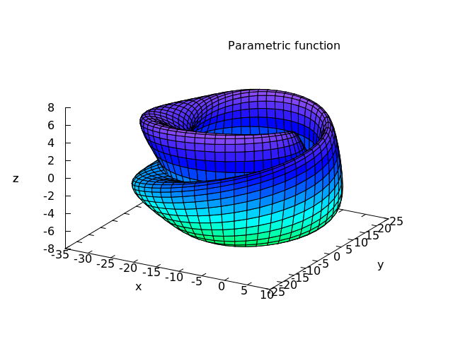
A parametric plot is defined by a list starting with the keyword parametric, followed by two expressions or function names and a range for the parameter. The range for the parameter must be a list with the name of the parameter followed by its minimum and maximum values: [param, min, max]. The plot will show the path traced out by the point with coordinates given by the two expressions or functions, as param increases from min to max.

A range for the vertical axis is an optional argument with the form: [y, min, max] (the keyword y is always used for the vertical axis). If that option is used, the plot will show that exact vertical range, independently of the values reached by the plot. If the vertical range is not specified, it will be set up according to the minimum and maximum values of the second coordinate of the plot points.

All other options should also be lists, starting with a keyword and followed by one or more values. See plot_options.

If there are several plots to be plotted, a legend will be written to identity each of the expressions. The labels that should be used in that legend can be given with the option legend. If that option is not used, Maxima will create labels from the expressions or function names.

Examples:

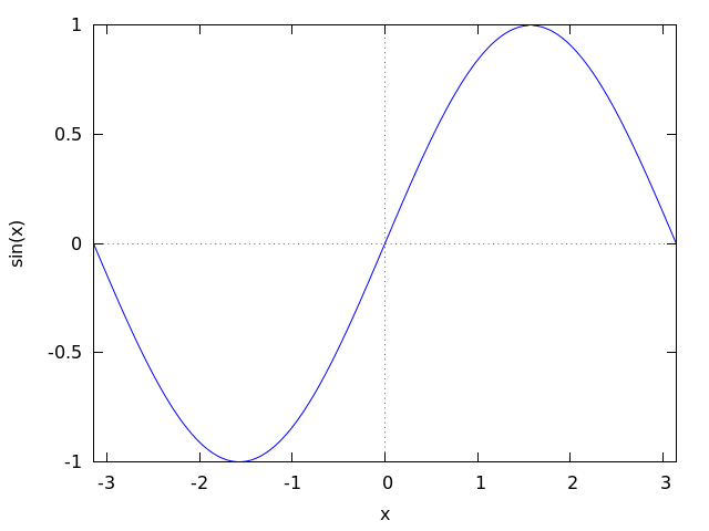
Plot of a common function:

(%i1) plot2d (sin(x), [x, -%pi, %pi])$

figures/plotting6

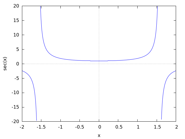
If the function grows too fast, it might be necessary to limit the values in the vertical axis using the y option:

(%i1) plot2d (sec(x), [x, -2, 2], [y, -20, 20])$

figures/plotting7

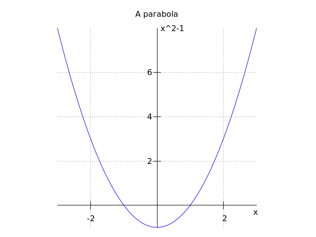
When the plot box is disabled, no labels are created for the axes. In that case, instead of using xlabel and ylabel to set the names of the axes, it is better to use option label, which allows more flexibility. Option yx_ratio is used to change the default rectangular shape of the plot; in this example the plot will fill a square.

(%i1) plot2d ( x^2 - 1, [x, -3, 3], [box, false], grid2d,
      [yx_ratio, 1], [axes, solid], [xtics, -2, 4, 2],
      [ytics, 2, 2, 6], [label, ["x", 2.9, -0.3],
      ["x^2-1", 0.1, 8]], [title, "A parabola"])$

figures/plotting8

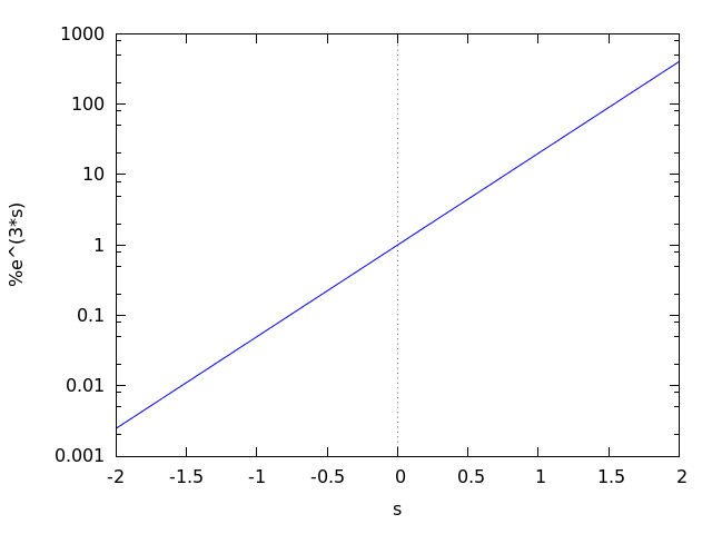
A plot with a logarithmic scale in the vertical axis:

(%i1) plot2d (exp(3*s), [s, -2, 2], logy)$

figures/plotting9

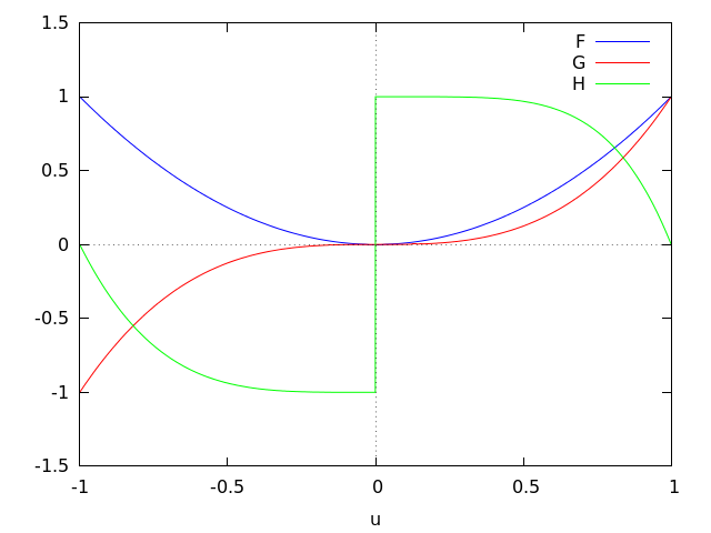
Plotting functions by name:

(%i1) F(x) := x^2 $
(%i2) :lisp (defun |$g| (x) (m* x x x))
$g
(%i2) H(x) := if x < 0 then x^4 - 1 else 1 - x^5 $
(%i3) plot2d ([F, G, H], [u, -1, 1], [y, -1.5, 1.5])$

figures/plotting10

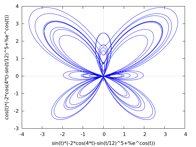
A plot of the butterfly curve, defined parametrically:

(%i1) r: (exp(cos(t))-2*cos(4*t)-sin(t/12)^5)$
(%i2) plot2d([parametric, r*sin(t), r*cos(t), [t, -8*%pi, 8*%pi]])$

figures/plotting11

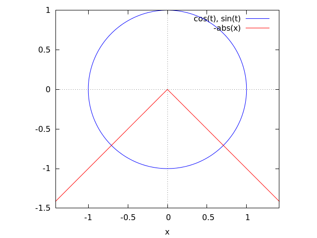
Plot of a circle, using its parametric representation, together with the function -|x|. The circle will only look like a circle if the scale in the two axes is the same, which is done with the option same_xy.

(%i1) plot2d([[parametric, cos(t), sin(t), [t,0,2*%pi]], -abs(x)],
         [x, -sqrt(2), sqrt(2)], same_xy)$

figures/plotting12

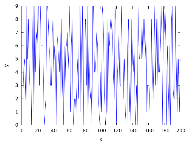
A plot of 200 random numbers between 0 and 9:

(%i1) plot2d ([discrete, makelist ( random(10), 200)])$

figures/plotting13

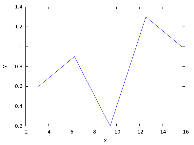
A plot of a discrete set of points, defining x and y coordinates separately:

(%i1) plot2d ([discrete, makelist(i*%pi, i, 1, 5),
                            [0.6, 0.9, 0.2, 1.3, 1]])$

figures/plotting14

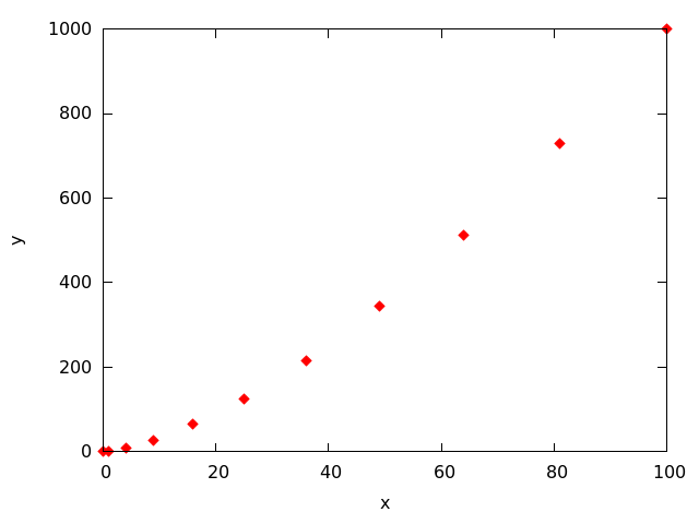
In the next example a table with three columns is saved in a file "data.txt" which is then read and the second and third column are plotted on the two axes:

(%i1) with_stdout ("data.txt", for x:0 thru 10 do
                             print (x, x^2, x^3))$
(%i2) data: read_matrix ("data.txt")$
(%i3) plot2d ([discrete, transpose(data)[2], transpose(data)[3]],
  [style,points], [point_type,diamond], [color,red])$

figures/plotting15

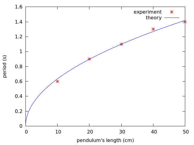
A plot of discrete data points together with a continuous function:

(%i1) xy: [[10, .6], [20, .9], [30, 1.1], [40, 1.3], [50, 1.4]]$
(%i2) plot2d([[discrete, xy], 2*%pi*sqrt(l/980)], [l,0,50],
        [style, points, lines], [color, red, blue],
        [point_type, asterisk],
        [legend, "experiment", "theory"],
        [xlabel, "pendulum's length (cm)"],
        [ylabel, "period (s)"])$

figures/plotting16

See also the section about Plotting Options.

Categories:  Plotting

Function: plot3d  
    plot3d (expr, x_range, y_range, …, options, …)  
    plot3d ([expr_1, …, expr_n], x_range, y_range, …, options, …)

Displays a plot of one or more surfaces defined as functions of two variables or in parametric form.

The functions to be plotted may be specified as expressions or function names. The mouse can be used to rotate the plot looking at the surface from different sides.

Examples:

Plot of a function of two variables:

(%i1) plot3d (u^2 - v^2, [u, -2, 2], [v, -3, 3], [grid, 100, 100],
        [mesh_lines_color,false])$

figures/plotting17

Use of the z option to limit a function that goes to infinity (in this case the function is minus infinity on the x and y axes); this also shows how to plot with only lines and no shading:

(%i1) plot3d ( log ( x^2*y^2 ), [x, -2, 2], [y, -2, 2], [z, -8, 4],
         [palette, false], [color, magenta])$

figures/plotting18

The infinite values of z can also be avoided by choosing a grid that does not fall on any points where the function is undefined, as in the next example, which also shows how to change the palette and how to include a color bar that relates colors to values of the z variable:

(%i1) plot3d (log (x^2*y^2), [x, -2, 2], [y, -2, 2],[grid, 29, 29],
       [palette, [gradient, red, orange, yellow, green]],
       color_bar, [xtics, 1], [ytics, 1], [ztics, 4],
       [color_bar_tics, 4])$

figures/plotting19

Two surfaces in the same plot. Ranges specific to one of the surfaces can be given by placing each expression and its ranges in a separate list; global ranges for the complete plot are also given after the functions definitions.

(%i1) plot3d ([[-3*x - y, [x, -2, 2], [y, -2, 2]],
   4*sin(3*(x^2 + y^2))/(x^2 + y^2), [x, -3, 3], [y, -3, 3]],
   [x, -4, 4], [y, -4, 4])$

figures/plotting20

Plot of a Klein bottle, defined parametrically:

(%i1) expr_1: 5*cos(x)*(cos(x/2)*cos(y)+sin(x/2)*sin(2*y)+3)-10$
(%i2) expr_2: -5*sin(x)*(cos(x/2)*cos(y)+sin(x/2)*sin(2*y)+3)$
(%i3) expr_3: 5*(-sin(x/2)*cos(y)+cos(x/2)*sin(2*y))$
(%i4) plot3d ([expr_1, expr_2, expr_3], [x, -%pi, %pi],
        [y, -%pi, %pi], [grid, 50, 50])$

figures/plotting21

Plot of a "spherical harmonic" function, using the predefined transformation, spherical_to_xyz to transform from spherical coordinates to rectangular coordinates. See the documentation for spherical_to_xyz.

(%i1) plot3d (sin(2*theta)*cos(phi), [theta, 0, %pi],
        [phi, 0, 2*%pi],
        [transform_xy, spherical_to_xyz], [grid,30,60],
   [legend,false])$

figures/plotting22

Use of the pre-defined function polar_to_xy to transform from cylindrical to rectangular coordinates. See the documentation for polar_to_xy.

(%i1) plot3d (r^.33*cos(th/3), [r,0,1], [th,0,6*%pi], [box, false],
   [grid, 12, 80], [transform_xy, polar_to_xy], [legend, false])$

figures/plotting23

Plot of a sphere using the transformation from spherical to rectangular coordinates. Option same_xyz is used to get the three axes scaled in the same proportion. When transformations are used, it is not convenient to eliminate the mesh lines, because Gnuplot will not show the surface correctly.

(%i1) plot3d ( 5, [theta, 0, %pi], [phi, 0, 2*%pi], same_xyz,
  [transform_xy, spherical_to_xyz], [mesh_lines_color,blue],
  [palette,[gradient,"#1b1b4e", "#8c8cf8"]], [legend, false])$

figures/plotting24

Definition of a function of two-variables using a matrix. Notice the single quote in the definition of the function, to prevent plot3d from failing when it realizes that the matrix will require integer indices.

(%i1) M: matrix([1,2,3,4], [1,2,3,2], [1,2,3,4], [1,2,3,3])$
(%i2) f(x, y) := float('M [round(x), round(y)])$
(%i3) plot3d (f(x,y), [x,1,4],[y,1,4],[grid,3,3],[legend,false])$

figures/plotting25

By setting the elevation equal to zero, a surface can be seen as a map in which each color represents a different level.

(%i1) plot3d (cos (-x^2 + y^3/4), [x,-4,4], [y,-4,4], [zlabel,""],
       [mesh_lines_color,false], [elevation,0], [azimuth,0],
       color_bar, [grid,80,80], [ztics,false], [color_bar_tics,1])$

figures/plotting26

See also the section about Plotting Options.

Categories:  Plotting

System variable: plot_options

This option is being kept for compatibility with older versions, but its use is deprecated. To set global plotting options, see their current values or remove options, use set_plot_option, get_plot_option and remove_plot_option.

Categories:  Plotting

Function: remove_plot_option (name)

Removes the default value of an option. The name of the option must be given.

See also set_plot_option, get_plot_option and the section on Plotting Options.

Categories:  Plotting

Function: set_plot_option (option)

Accepts any of the options listed in the section Plotting Options, and saves them for use in plotting commands. The values of the options set in each plotting command will have precedence, but if those options are not given, the default values set with this function will be used.

set_plot_option evaluates its argument and returns the complete list of options (after modifying the option given). If called without any arguments, it will simply show the list of current default options.

See also remove_plot_option, get_plot_option and the section on Plotting Options.

Example:

Modification of the grid values.

(%i1) set_plot_option ([grid, 30, 40]);
(%o1) [[plot_format, gnuplot_pipes], [grid, 30, 40], 
[run_viewer, true], [axes, true], [nticks, 29], [adapt_depth, 5], 
[color, blue, red, green, magenta, black, cyan], 
[point_type, bullet, box, triangle, plus, times, asterisk], 
[palette, [gradient, green, cyan, blue, violet], 
[gradient, magenta, violet, blue, cyan, green, yellow, orange, 
red, brown, black]], [gnuplot_preamble, ], [gnuplot_term, default]]

Categories:  Plotting

System function: spherical_to_xyz

It can be given as value for the transform_xy option of plot3d. Its effect will be to interpret the two independent variables and the function in plot3d as the spherical coordinates of a point (first, the angle with the z axis, then the angle of the xy projection with the x axis and finally the distance from the origin) and transform them into x, y and z coordinates.

Categories:  Plotting


[ < ] [ > ]   [ << ] [ Up ] [ >> ]         [Top] [Contents] [Index] [ ? ]

12.4 Plotting Options

All options consist of a list starting with one of the keywords in this section, followed by one or more values. Some of the options may have different effects in different plotting commands as it will be pointed out in the following list. The options that accept among their possible values true or false, can also be set to true by simply writing their names. For instance, typing logx as an option is equivalent to writing [logx, true].

Plot option: adapt_depth [adapt_depth, integer]

Default value: 5

The maximum number of splittings used by the adaptive plotting routine.

Categories:  Plotting

Plot option: axes [axes, symbol]

Default value: true

Where symbol can be either true, false, x, y or solid. If false, no axes are shown; if equal to x or y only the x or y axis will be shown; if it is equal to true, both axes will be shown and solid will show the two axes with a solid line, rather than the default broken line. This option does not have any effect in the 3 dimensional plots.

Categories:  Plotting

Plot option: azimuth [azimuth, number]

Default value: 30

A plot3d plot can be thought of as starting with the x and y axis in the horizontal and vertical axis, as in plot2d, and the z axis coming out of the screen. The z axis is then rotated around the x axis through an angle equal to elevation and then the new xy plane is rotated around the new z axis through an angle azimuth. This option sets the value for the azimuth, in degrees.

See also elevation.

Categories:  Plotting

Plot option: box [box, symbol]

Default value: true

If set to true, a bounding box will be drawn for the plot; if set to false, no box will be drawn.

Categories:  Plotting

Plot option: color [color, color_1, …, color_n]

In 2d plots it defines the color (or colors) for the various curves. In plot3d, it defines the colors used for the mesh lines of the surfaces, when no palette is being used.

If there are more curves or surfaces than colors, the colors will be repeated in sequence. The valid colors are red, green, blue, magenta, cyan, yellow, orange, violet, brown, gray, black, white, or a string starting with the character # and followed by six hexadecimal digits: two for the red component, two for green component and two for the blue component. If the name of a given color is unknown color, black will be used instead.

Categories:  Plotting

Plot option: color_bar [color_bar, symbol]

Default value: false in plot3d, true in mandelbrot and julia

Where symbol can be either true or false. If true, whenever plot3d, mandelbrot or julia use a palette to represent different values, a box will be shown on the right, showing the corresponding between colors and values.

Categories:  Plotting

Plot option: color_bar_tics [color_bar_tics, x1, x2, x3]

Defines the values at which a mark and a number will be placed in the color bar. The first number is the initial value, the second the increments and the third is the last value where a mark is placed. The second and third numbers can be omitted. When only one number is given, it will be used as the increment from an initial value that will be chosen automatically.

Categories:  Plotting

Plot option: elevation [elevation, number]

Default value: 60

A plot3d plot can be thought of as starting with the x and y axis in the horizontal and vertical axis, as in plot2d, and the z axis coming out of the screen. The z axis is then rotated around the x axis through an angle equal to elevation and then the new xy plane is rotated around the new z axis through an angle azimuth. This option sets the value for the azimuth, in degrees.

See also azimuth.

Categories:  Plotting

Plot option: grid [grid, integer, integer]

Default value: 30, 30

Sets the number of grid points to use in the x- and y-directions for three-dimensional plotting or for the julia and mandelbrot programs.

Categories:  Plotting

Plot option: grid2d [grid, value]

Default value: false

Shows a grid of lines on the xy plane. The points where the grid lines are placed are the same points where tics are marked in the x and y axes, which can be controlled with the xtics and ytics options.

Categories:  Plotting

Plot option: iterations [grid, value]

Default value: 9

Number of iterations made by the programs mandelbrot and julia.

Categories:  Plotting

Plot option: label [label, [string, x, y], …]

Writes one or several labels in the points with x, y coordinates indicated after each label.

Categories:  Plotting

Plot option: legend  
    legend [legend, string_1, …, string_n]  
    legend [legend, false]

It specifies the labels for the plots when various plots are shown. If there are more plots than the number of labels given, they will be repeated. If given the value false, no legends will be shown. By default, the names of the expressions or functions will be used, or the words discrete1, discrete2, …, for discrete sets of points.

Categories:  Plotting

Plot option: logx [logx, value]

Makes the horizontal axes to be scaled logarithmically. It can be either true or false.

Categories:  Plotting

Plot option: logy [logy, value]

Makes the vertical axes to be scaled logarithmically. It can be either true or false.

Categories:  Plotting

Plot option: mesh_lines_color [mesh_lines_color, color]

Default value: black

It sets the color used by plot3d to draw the mesh lines, when a palette is being used. It accepts the same colors as for the option color (see the list of allowed colors in color). It can also be given a value false to eliminate completely the mesh lines.

Categories:  Plotting

Plot option: nticks [nticks, integer]

Default value: 29

When plotting functions with plot2d, it is gives the initial number of points used by the adaptive plotting routine for plotting functions. When plotting parametric functions with plot3d, it sets the number of points that will be shown for the plot.

Categories:  Plotting

Plot option: palette  
    palette [palette, [palette_1], …, [palette_n]]  
    palette [palette, false]

It can consist of one palette or a list of several palettes. Each palette is a list with a keyword followed by values. If the keyword is gradient, it should be followed by a list of valid colors.

If the keyword is hue, saturation or value, it must be followed by 4 numbers. The first three numbers, which must be between 0 and 1, define the hue, saturation and value of a basic color to be assigned to the minimum value of z. The keyword specifies which of the three attributes (hue, saturation or value) will be increased according to the values of z. The last number indicates the increase corresponding to the maximum value of z. That last number can be bigger than 1 or negative; the corresponding values of the modified attribute will be rounded modulo 1.

Gnuplot only uses the first palette in the list; xmaxima will use the palettes in the list sequentially, when several surfaces are plotted together; if the number of palettes is exhausted, they will be repeated sequentially.

The color of the mesh lines will be given by the option mesh_lines_color. If palette is given the value false, the surfaces will not be shaded but represented with a mesh of curves only. In that case, the colors of the lines will be determined by the option color.

Categories:  Plotting

Plot option: plot_format [plot_format, format]

Default value: gnuplot, in Windows systems, or gnuplot_pipes in other systems.

Where format is one of the following: gnuplot, xmaxima, mgnuplot or gnuplot_pipes.

It sets the format to be used for plotting.

Categories:  Plotting

Plot option: plot_realpart [plot_realpart, symbol]

Default value: false

If set to true, the functions to be plotted will be considered as complex functions whose real value should be plotted; this is equivalent to plotting realpart(function). If set to false, nothing will be plotted when the function does not give a real value. For instance, when x is negative, log(x) gives a complex value, with real value equal to log(abs(x)); if plot_realpart were true, log(-5) would be plotted as log(5), while nothing would be plotted if plot_realpart were false.

Categories:  Plotting

Plot option: point_type [point_type, type_1, …, type_n]

In gnuplot, each set of points to be plotted with the style "points" or "linespoints" will be represented with objects taken from this list, in sequential order. If there are more sets of points than objects in this list, they will be repeated sequentially. The possible objects that can be used are: bullet, circle, plus, times, asterisk, box, square, triangle, delta, wedge, nabla, diamond, lozenge.

Categories:  Plotting

Plot option: pdf_file [pdf_file, file_name]

Saves the plot into a PDF file with name equal to file_name, rather than showing it in the screen. By default, the file will be created in the directory defined by the variable maxima_tempdir, unless file_name contains the character "/", in which case it will be assumed to contain the complete path where the file should be created. The value of maxima_tempdir can be changed to save the file in a different directory. When the option gnuplot_pdf_term_command is also given, it will be used to set up Gnuplot's PDF terminal; otherwise, Gnuplot's pdfcairo terminal will be used with solid colored lines of width 3, plot size of 17.2 cm by 12.9 cm and font of 18 points.

Categories:  Plotting

Plot option: png_file [png_file, file_name]

Saves the plot into a PNG graphics file with name equal to file_name, rather than showing it in the screen. By default, the file will be created in the directory defined by the variable maxima_tempdir, unless file_name contains the character "/", in which case it will be assumed to contain the complete path where the file should be created. The value of maxima_tempdir can be changed to save the file in a different directory. When the option gnuplot_png_term_command is also given, it will be used to set up Gnuplot's PNG terminal; otherwise, Gnuplot's pngcairo terminal will be used, with a font of size 12.

Categories:  Plotting

Plot option: ps_file [ps_file, file_name]

Saves the plot into a Postscript file with name equal to file_name, rather than showing it in the screen. By default, the file will be created in the directory defined by the variable maxima_tempdir, unless file_name contains the character "/", in which case it will be assumed to contain the complete path where the file should be created. The value of maxima_tempdir can be changed to save the file in a different directory. When the option gnuplot_ps_term_command is also given, it will be used to set up Gnuplot's Postscript terminal; otherwise, Gnuplot's postscript terminal will be used with the EPS option, solid colored lines of width 2, plot size of 16.4 cm by 12.3 cm and font of 24 points.

Categories:  Plotting

Plot option: run_viewer [run_viewer, symbol]

This option is only used when the plot format is gnuplot and the terminal is default or when the Gnuplot terminal is set to dumb (see gnuplot_term) and can have a true or false value.

If the terminal is default, a file maxout_xxx.gnuplot (or other name specified with gnuplot_out_file) is created with the gnuplot commands necessary to generate the plot. Option run_viewer controls whether or not Gnuplot will be launched to execute those commands and show the plot.

If the terminal is default, gnuplot is run to execute the commands in maxout_xxx.gnuplot, producing another file maxplot.txt (or other name specified with gnuplot_out_file). Option run_viewer controls whether or not that file, with an ASCII representation of the plot, will be shown in the Maxima or Xmaxima console.

The default value for this option is true, making the plots to be shown in either the console or a separate graphics window.

Categories:  Plotting

Plot option: same_xy [same_xy , value]

It can be either true or false. If true, the scales used in the x and y axes will be the same, in either 2d or 3d plots. See also yx_ratio.

Categories:  Plotting

Plot option: same_xyz [same_xyz , value]

It can be either true or false. If true, the scales used in the 3 axes of a 3d plot will be the same.

Categories:  Plotting

Plot option: style  
    style [style, type_1, …, type_n]  
    style [style, [style_1], …, [style_n]]

The styles that will be used for the various functions or sets of data in a 2d plot. The word style must be followed by one or more styles. If there are more functions and data sets than the styles given, the styles will be repeated. Each style can be either lines for line segments, points for isolated points, linespoints for segments and points, or dots for small isolated dots. Gnuplot accepts also an impulses style.

Each of the styles can be enclosed inside a list with some additional parameters. lines accepts one or two numbers: the width of the line and an integer that identifies a color. The default color codes are: 1: blue, 2: red, 3: magenta, 4: orange, 5: brown, 6: lime and 7: aqua. If you use Gnuplot with a terminal different than X11, those colors might be different; for example, if you use the option [gnuplot_term, ps], color index 4 will correspond to black, instead of orange.

points accepts one two or three parameters; the first parameter is the radius of the points, the second parameter is an integer that selects the color, using the same code used for lines and the third parameter is currently used only by Gnuplot and it corresponds to several objects instead of points. The default types of objects are: 1: filled circles, 2: open circles, 3: plus signs, 4: x, 5: *, 6: filled squares, 7: open squares, 8: filled triangles, 9: open triangles, 10: filled inverted triangles, 11: open inverted triangles, 12: filled lozenges and 13: open lozenges.

linespoints accepts up to four parameters: line width, points radius, color and type of object to replace the points.

See also color and point_type.

Categories:  Plotting

Plot option: svg_file [svg_file, file_name]

Saves the plot into an SVG file with name equal to file_name, rather than showing it in the screen. By default, the file will be created in the directory defined by the variable maxima_tempdir, unless file_name contains the character "/", in which case it will be assumed to contain the complete path where the file should be created. The value of maxima_tempdir can be changed to save the file in a different directory. When the option gnuplot_svg_term_command is also given, it will be used to set up Gnuplot's SVG terminal; otherwise, Gnuplot's svg terminal will be used with font of 14 points.

Categories:  Plotting

Plot option: t [t, min, max]

Default range for parametric plots.

Categories:  Plotting

Plot option: title [title, text]

Defines a title that will be written at the top of the plot.

Categories:  Plotting

Plot option: transform_xy [transform_xy, symbol]

Where symbol is either false or the result obtained by using the function transform_xy. If different from false, it will be used to transform the 3 coordinates in plot3d.

See make_transform, polar_to_xy and spherical_to_xyz.

Categories:  Plotting

Plot option: x [x, min, max]

When used as the first option in a plot2d command (or any of the first two in plot3d), it indicates that the first independent variable is x and it sets its range. It can also be used again after the first option (or after the second option in plot3d) to define the effective horizontal domain that will be shown in the plot.

Categories:  Plotting

Plot option: xlabel [xlabel, string]

Specifies the string that will label the first axis; if this option is not used, that label will be the name of the independent variable, when plotting functions with plot2d or implicit_plot, or the name of the first variable, when plotting surfaces with plot3d or contours with contour_plot, or the first expression in the case of a parametric plot. It can not be used with set_plot_option.

Categories:  Plotting

Plot option: xtics [xtics, x1, x2, x3]

Defines the values at which a mark and a number will be placed in the x axis. The first number is the initial value, the second the increments and the third is the last value where a mark is placed. The second and third numbers can be omitted. When only one number is given, it will be used as the increment from an initial value that will be chosen automatically.

Categories:  Plotting

Plot option: xy_scale [xy_scale, sx, sy]

In a 2d plot, it defines the ratio of the total size of the Window to the size that will be used for the plot. The two numbers given as arguments are the scale factors for the x and y axes.

Categories:  Plotting

Plot option: y [y, min, max]

When used as one of the first two options in plot3d, it indicates that one of the independent variables is y and it sets its range. Otherwise, it defines the effective domain of the second variable that will be shown in the plot.

Categories:  Plotting

Plot option: ylabel [ylabel, string]

Specifies the string that will label the second axis; if this option is not used, that label will be "y", when plotting functions with plot2d or implicit_plot, or the name of the second variable, when plotting surfaces with plot3d or contours with contour_plot, or the second expression in the case of a parametric plot. It can not be used with set_plot_option.

Categories:  Plotting

Plot option: ytics [ytics, y1, y2, y3]

Defines the values at which a mark and a number will be placed in the y axis. The first number is the initial value, the second the increments and the third is the last value where a mark is placed. The second and third numbers can be omitted. When only one number is given, it will be used as the increment from an initial value that will be chosen automatically

Categories:  Plotting

Plot option: yx_ratio [yx_ratio, r]

In a 2d plot, the ratio between the vertical and the horizontal sides of the rectangle used to make the plot. See also same_xy.

Categories:  Plotting

Plot option: z [z, min, max]

Used in plot3d to set the effective range of values of z that will be shown in the plot.

Categories:  Plotting

Plot option: zlabel [zlabel, string]

Specifies the string that will label the third axis, when using plot3d. If this option is not used, that label will be "z", when plotting surfaces, or the third expression in the case of a parametric plot. It can not be used with set_plot_option and it will be ignored by plot2d and implicit_plot.

Categories:  Plotting

Plot option: zmin [zmin, z]

In 3d plots, the value of z that will be at the bottom of the plot box.

Categories:  Plotting


[ < ] [ > ]   [ << ] [ Up ] [ >> ]         [Top] [Contents] [Index] [ ? ]

12.5 Gnuplot Options

There are several plot options specific to gnuplot. All of them consist of a keyword (the name of the option), followed by a string that should be a valid gnuplot command, to be passed directly to gnuplot. In most cases, there exist a corresponding plotting option that will produce a similar result and whose use is more recommended than the gnuplot specific option.

Plot option: gnuplot_term [gnuplot_term, terminal_name]

Sets the output terminal type for gnuplot. The argument terminal_name can be a string or one of the following 3 special symbols

Categories:  Plotting

Plot option: gnuplot_out_file [gnuplot_out_file, file_name]

It can be used to replace the default name for the file that contains the commands that will interpreted by gnuplot, when the terminal is set to default, or to replace the default name of the graphic file that gnuplot creates, when the terminal is different from default. If it contains one or more slashes, "/", the name of the file will be left as it is; otherwise, it will be appended to the path of the temporary directory. The complete name of the files created by the plotting commands is always sent as output of those commands so they can be seen if the command is ended by semi-colon.

When used in conjunction with the gnuplot_term option, it can be used to save the plot in a file, in one of the graphic formats supported by Gnuplot. To create PNG, PDF, Postscript or SVG, it is easier to use options png_file, pdf_file, ps_file, or svg_file.

Categories:  Plotting

Plot option: gnuplot_pm3d [gnuplot_pm3d, value]

With a value of false, it can be used to disable the use of PM3D mode, which is enabled by default.

Categories:  Plotting

Plot option: gnuplot_preamble [gnuplot_preamble, string]

This option inserts gnuplot commands before any other commands sent to Gnuplot. Any valid gnuplot commands may be used. Multiple commands should be separated with a semi-colon. See also gnuplot_postamble.

Categories:  Plotting

Plot option: gnuplot_postamble [gnuplot_postamble, string]

This option inserts gnuplot commands after other commands sent to Gnuplot and right before the plot command is sent. Any valid gnuplot commands may be used. Multiple commands should be separated with a semi-colon. See also gnuplot_preamble.

Categories:  Plotting

Plot option: gnuplot_default_term_command

[gnuplot_default_term_command, command]

The gnuplot command to set the terminal type for the default terminal. It this option is not set, the command used will be: "set term wxt size 640,480 font \",12\"; set term pop".

Categories:  Plotting

Plot option: gnuplot_dumb_term_command

[gnuplot_dumb_term_command, command]

The gnuplot command to set the terminal type for the dumb terminal. It this option is not set, the command used will be: "set term dumb 79 22", which makes the text output 79 characters by 22 characters.

Categories:  Plotting

Plot option: gnuplot_pdf_term_command [gnuplot_pdf_term_command, command]

The gnuplot command to set the terminal type for the PDF terminal. If this option is not set, the command used will be: "set term pdfcairo color solid lw 3 size 17.2 cm, 12.9 cm font \",18\"". See the gnuplot documentation for more information.

Categories:  Plotting

Plot option: gnuplot_png_term_command [gnuplot_png_term_command, command]

The gnuplot command to set the terminal type for the PNG terminal. If this option is not set, the command used will be: "set term pngcairo font \",12\"". See the gnuplot documentation for more information.

Categories:  Plotting

Plot option: gnuplot_ps_term_command [gnuplot_ps_term_command, command]

The gnuplot command to set the terminal type for the PostScript terminal. If this option is not set, the command used will be: "set term postscript eps color solid lw 2 size 16.4 cm, 12.3 cm font \",24\"". See the gnuplot documentation for set term postscript for more information.

Categories:  Plotting

Plot option: gnuplot_svg_term_command [gnuplot_svg_term_command, command]

The gnuplot command to set the terminal type for the SVG terminal. If this option is not set, the command used will be: "set term svg font \",14\"". See the gnuplot documentation for more information.

Categories:  Plotting

Plot option: gnuplot_curve_titles

This is an obsolete option that has been replaced legend described above.

Categories:  Plotting

Plot option: gnuplot_curve_styles

This is an obsolete option that has been replaced by style.

Categories:  Plotting


[ < ] [ > ]   [ << ] [ Up ] [ >> ]         [Top] [Contents] [Index] [ ? ]

12.6 Gnuplot_pipes Format Functions

Function: gnuplot_start ()

Opens the pipe to gnuplot used for plotting with the gnuplot_pipes format. Is not necessary to manually open the pipe before plotting.

Categories:  Plotting

Function: gnuplot_close ()

Closes the pipe to gnuplot which is used with the gnuplot_pipes format.

Categories:  Plotting

Function: gnuplot_restart ()

Closes the pipe to gnuplot which is used with the gnuplot_pipes format and opens a new pipe.

Categories:  Plotting

Function: gnuplot_replot  
    gnuplot_replot ()  
    gnuplot_replot (s)

Updates the gnuplot window. If gnuplot_replot is called with a gnuplot command in a string s, then s is sent to gnuplot before reploting the window.

Categories:  Plotting

Function: gnuplot_reset ()

Resets the state of gnuplot used with the gnuplot_pipes format. To update the gnuplot window call gnuplot_replot after gnuplot_reset.

Categories:  Plotting


[ << ] [ >> ]           [Top] [Contents] [Index] [ ? ]

This document was generated by Raymond Toy on May, 22 2016 using texi2html 1.76.